Reading Weather Patterns — Practice · Grade 9 Science
Chapter: Atmosphere & WeatherWhat this practice covers
By the end of Reading Weather Patterns you should be able to:
- I can identify H, L, fronts, isobars, and station models on a weather map.
- I can use a barometric pressure trend to predict whether weather will improve or worsen.
- I can explain why weather in the mid-latitudes, including New York, generally moves from west to east.
11 questions, multiple choice, numeric and written answer, each with a worked explanation.
Vocabulary used: isobar, station model, meteorologist, prevailing westerlies, relative humidity, dew point.
Problem 1
- Isobar
- Isotherm
- Front
- Station model
Answer and explanation
Isobar
Isobars connect points of equal air pressure — 'iso' means equal and 'bar' refers to pressure.
Problem 2
- Barometer
- Anemometer
- Hygrometer
- Rain gauge
Answer and explanation
Barometer
A barometer measures air pressure; an anemometer measures wind speed, a hygrometer measures humidity, and a rain gauge measures precipitation.
Problem 3
- From west to east
- From east to west
- From north to south only
- Randomly, with no general pattern
Answer and explanation
From west to east
The prevailing westerlies and the jet stream generally steer mid-latitude weather from west to east.
Problem 4
- Strong winds, due to a big pressure difference over a short distance
- Calm winds, because the pressure is very steady
- An approaching heat wave with no wind
- That the map has an error
Answer and explanation
Strong winds, due to a big pressure difference over a short distance
Tightly packed isobars mean pressure changes quickly over a short distance, and bigger pressure differences drive stronger winds.
Problem 5
Answer and explanation
18 mb
1020 − 1002 = 18 mb. That's a fairly rapid fall, often a sign that stormier weather is on the way.
Problem 6
Answer and explanation
30 km/h over the measured interval; a later arrival estimate needs continued observations.
Average speed=180/6=30 km/h.
Future speed or direction can change, so straight extrapolation is an assumption.
Response criteria
- Use the stated conditions.
- Show the evidence or calculation.
- Explain the conclusion and any stated limitation.
Problem 7
Hints
A forecast is conditional and updated with new evidence.
Answer and explanation
Distance to the location and movement speed/direction over successive images, with allowance for growth or decay.
Problem 8
Hints
State what the supplied observations or conditions establish, and separate that from any assumption.
Answer and explanation
Initial-state uncertainty and evolving interactions can amplify differences in predictions.
Problem 9
Answer and explanation
1.5 h at 40 km/h and 2 h at 30 km/h, assuming steady speed along the stated path. Actual movement can evolve.
The curves share an initial position and direction but differ in slope. The vertical axis is travel distance, not temperature or precipitation probability.
1.5 h at 40 km/h and 2 h at 30 km/h, assuming steady speed along the stated path. Actual movement can evolve.
Response criteria
- Read the labeled quantities, reference frame or objects correctly.
- Explain the relation between the visual evidence and the mechanism.
- Keep the drawing’s stated assumptions and limits in the conclusion.
Problem 10
Answer and explanation
A gives 3 h and B 2 h. Record the forecast issue time, defined passage indicator/location and predicted intervals, then compare with later observations using the original criteria. Changing criteria after the event undermines verification.
A gives 3 h and B 2 h. Record the forecast issue time, defined passage indicator/location and predicted intervals, then compare with later observations using the original criteria. Changing criteria after the event undermines verification.
Response criteria
- Use the stated measurements or conditions, with correct units.
- Connect the result to the physical mechanism or evidence relationship.
- Identify the assumption, model limit or further evidence requested.
Problem 11
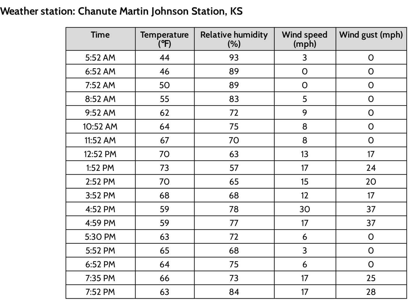
Answer and explanation
Temperature changes from 68 to 59 °F: −9 °F, equivalent to −5 °C. Relative humidity changes from 68% to 78%: +10 percentage points, not a 10% relative increase. Wind speed changes from 12 to 30 mph: +18 mph. The observations support a changing atmospheric situation at the named station; mapped front/pressure, wind direction, moisture and event-location evidence would help test causes. A humidity increase alone does not prove more water vapor, because saturation conditions change with temperature.
Read matching times and the correct source columns before subtracting.
Subtract later minus earlier: 59−68 = −9 °F; multiply the difference by 5/9 to obtain −5 °C. Do not subtract 32 when converting a temperature difference.
Compute 78−68 = 10 percentage points and 30−12 = 18 mph; gusts are a separate column.
State the station scale and time interval, then request independent mapped/process evidence rather than claim a unique cause.
Response criteria
- All changes use later minus earlier and retain correct units.
- Temperature-difference conversion and percentage-point distinction are correct.
- The inference is limited to the stated record and identifies evidence needed for a causal explanation.