A First Taste of Algorithms · Order, and Its Price
The halver returns
Chapter 3 already built the alternative: merge sort — split, sort each half, merge — with its bill read off the tree: every level’s merges touch n cards, log₂ n levels, about n log₂ n element-steps. (A lineage note worth one sentence: when John von Neumann sketched programs for the first stored-program computer in 1945, among the very first things he wrote out was merge sort. The halver is as old as the machines themselves.)
Now race them in the counted currency, worst case against worst case, and read the gap as it opens:
| n | insertion (comparisons) | merge (element-steps) |
|---|---|---|
| 8 | 28 | 24 |
| 32 | 496 | 160 |
| 128 | 8,128 | 896 |
| 512 | 130,816 | 4,608 |
| 2,048 | 2,096,128 | 22,528 |
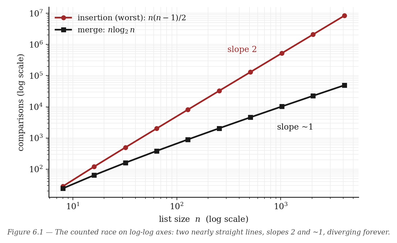
Figure 6.1 — The counted race on log-log axes: two nearly straight lines, slopes 2 and ~1, diverging forever. In this currency the halver never loses.
At a deck of 8 the two are neighbors. At 2,048 the plodder pays ninety times more, and every doubling of the deck doubles the ratio again. In the counted currency, the halver never loses and never looks back — Lab 6 plots this table and the gap becomes a pair of diverging straight lines. (Then why does insertion sort exist in every real library on Earth? Because clocks are not counts. Lab 6’s second experiment times both on your machine and finds a neighborhood — small n — where the plodder’s low overhead wins the clock while losing the count. Constants, the thing our counting openly declines to chase, own the small-n neighborhood; the count owns everywhere else. This is Chapter 1’s confession, audited and confirmed.)
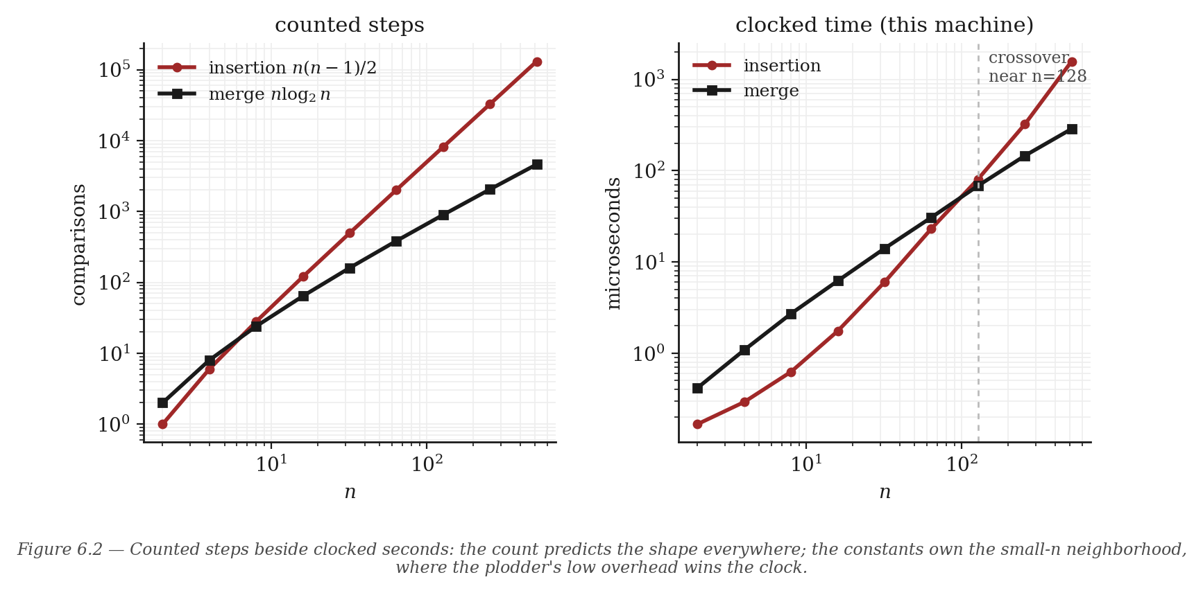
Figure 6.2 — Counted steps beside clocked seconds: the count predicts the shape everywhere; the constants own the small-n neighborhood, where the plodder’s low overhead wins the clock.
Names for the shapes, at last
Six chapters of tables have earned you the right to some professional shorthand. You have met, repeatedly, costs that grow like log n, like n, like n log n, like n², like 2ⁿ — and what mattered every single time was the shape, never the constant: not “496 comparisons” but “quadruples when n doubles.”
The notation: a cost grows as O(f(n)) — read “big-oh of f” — if, for large n, it is at most a constant multiple of f(n). It grows as Ω(f(n)) if it is at least a constant multiple. Θ(f(n)) claims both: the shape, exactly. So insertion sort’s worst case is Θ(n²); merge sort’s is Θ(n log n); binary search is Θ(log n); the amnesiac staircase was exponential and the notebook made it Θ(n).
Three honest remarks, because notation is where understanding goes to hide:
- O is a ceiling, not a destination. “Insertion sort is O(n²)” promises it never exceeds that shape; it does not promise to reach it. On an already-sorted deck, insertion runs in n − 1 steps. Saying “O(n²), so it takes about n² steps” is a misreading you will now hear weekly for the rest of your life; correct it gently.
- The dropped constants are real. Θ tells you who wins the race eventually; the clocked crossover tells you the constants pick the winner at small n. Both are facts; the notation simply chooses, openly, to track the first.
- We waited on purpose. This notation in Chapter 1 would have been vocabulary; in Chapter 6 it is bookkeeping for tables you built yourself. Notation should always arrive in arrears.
All 32 chapters of A First Taste of Algorithms · Foundations · All courses