A First Taste of Algorithms · The Algorithm That Flips Coins

The move

So stop being predictable. Choose the pivot by flipping coins — uniformly at random from the current list, fresh randomness at every level.

Feel precisely what changed, because it is a shift in the logic, not the code. Before: the adversary picks the input after reading your rule, so there exists a bad input. After: the adversary still picks any input it likes — sorted, reversed, crafted with infinite malice — but your coins are flipped afterward, and the coins do not read lists. Against every input, most pivots are decent (half the items split off at least a quarter of the list — mediocrity is abundant). There is no longer such a thing as a bad input; there is only bad luck, and bad luck, unlike a bad input, cannot be arranged by anyone.

The worst case did not vanish — be honest about this. The coins could come up cruel every time, and the n² bill would arrive; Problem 3.1 makes you stare at that possibility. What changed is its status: from “the adversary’s certainty” to “an improbability on every input, of the same kind as shuffling a deck into perfect order.” We have traded a guarantee for a gamble. The rest of the chapter is about why this particular gamble deserves your trust — which requires knowing, honestly, what “fast on average” means.

What an average promises

Expected value is the average of the outcomes weighted by their probabilities — the long-run average if you played forever. A die’s expected roll is (1+2+3+4+5+6)/6 = 3.5: a number the die never shows, and yet the most useful single fact about it.

The tool that makes expectation compute is one fact, modest-looking and inexhaustible — linearity: the expectation of a sum is the sum of the expectations, always, even when the pieces influence each other. No independence required, no fine print. Watch it demolish a problem that looks hopeless. The hat-check story: n people check their hats; the clerk loses the tickets and returns hats at random. On average, how many people get their own hat back?

The full analysis looks dreadful — whether you get your hat affects whether I get mine. Linearity ignores the entanglement. Person i gets their own hat with probability 1/n (one right hat among n, symmetry). The number of lucky people is a sum of n such person-by-person events, so its expectation is the sum of the pieces: n × (1/n) = 1. One lucky person on average — for ten hats, for a million hats, for any n whatsoever. The interactions, which terrified us, were never asked to testify. That is linearity’s standing offer: decompose the quantity into small events, price each alone, add. It is the table method’s spirit — refuse the whole, price the pieces — applied to chance, and it is the workhorse of every average in this subject.

Applied to quicksort (the full derivation is the deep water; here is its shape): decompose the total comparisons into pair-by-pair events — do items i and j ever get compared? They do exactly when one of them is the first pivot chosen from the stretch of items between them, which for distant pairs is unlikely; price each pair, add them all, and the sum comes out near 2n ln n — the n log n shape, with a particular constant, as a theorem about the average. For n = 256 that is a few thousand comparisons against a worst case of 32,640.

But an average alone can mislead (the hat-check average is 1 whether the outcomes are steady or wild), so the lab does the thing this book always does: it measures the whole distribution. Two thousand independent runs of randomized quicksort on the same input, every comparison counted, all of it poured into your first histogram — and the picture is the argument: a tight hill near the mean, thin tails, and the worst case so far to the right it cannot share the page. The gamble is not a coin flip between fast and slow; it is fast with overwhelming concentration, and you will have seen it with your own instrument rather than taken it on faith.

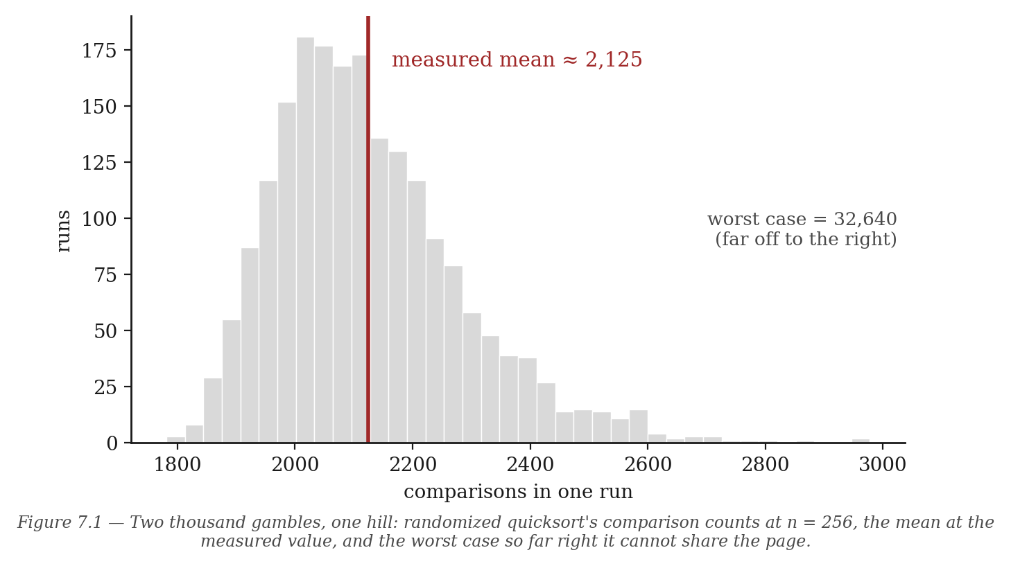
Figure 7.1 — Two thousand gambles, one hill: randomized quicksort’s comparison counts at n = 256, the mean at the measured 2,125, and the worst case so far right it cannot share the page.

A human moment

Computing with deliberate randomness was born in convalescence, over a card game. In 1946 Stanisław Ulam — recovering from a severe illness, playing endless rounds of solitaire — asked himself what fraction of solitaire deals are winnable. The honest combinatorics was hopeless. Then the lazier, deeper thought: deal a hundred random games and count. Back at Los Alamos, Ulam and John von Neumann (his second appearance in two chapters — the man is unavoidable) realized the trick was general: problems too tangled to solve exactly — neutrons rattling through a bomb core, integrals with no formula — could be sampled instead, on the new electronic computers, with manufactured randomness. The approach needed a code name, and their colleague Nicholas Metropolis supplied one from family gossip: Ulam had an uncle who was forever borrowing money to gamble at Monte Carlo. The name stuck to the method, then to a whole way of computing. Within it sits this chapter’s lesson in miniature: when exact analysis closes its door, an honest die and a fast counter open a window — and the window, used carefully, can be made as trustworthy as the door.

All 32 chapters of A First Taste of Algorithms · Foundations · All courses