Calculus I · Adding Up the Infinite

Riemann sums: approximate with rectangles, then take the limit

We cannot find the area under a curve directly, so we approximate it with shapes we can measure — rectangles — and then make the approximation exact with a limit. (This is the identical strategy from Chapter 3, where we approximated a slope with a secant line and took the limit. Calculus has essentially one idea, and this is its second great use.)

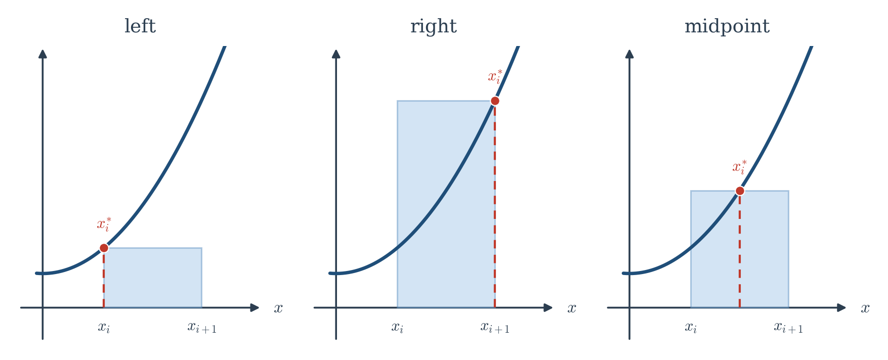
To estimate the area under $f$ on $[a,b]$: chop the interval into $n$ equal slices, each of width $\Delta x = \dfrac{b-a}{n}$. On each slice, build a rectangle whose height is the value of $f$ at some sample point $x_i$ in that slice. The rectangle areas are $f(x_i)\,\Delta x$, and their sum approximates the total area:

$$\text{Area} \approx \sum_{i=1}^{n} f(x_i)\,\Delta x.$$

This is a Riemann sum. Using the left edge of each slice as the sample point gives a left sum, the right edge a right sum, the middle a midpoint sum — and for a great many functions, all of them close in on the same number as the rectangles get thinner. (Figure 10.2: the region under a curve filled with rectangles, shown at $n=4$, $n=8$, $n=16$ — the staircase hugging the curve more tightly each time.)

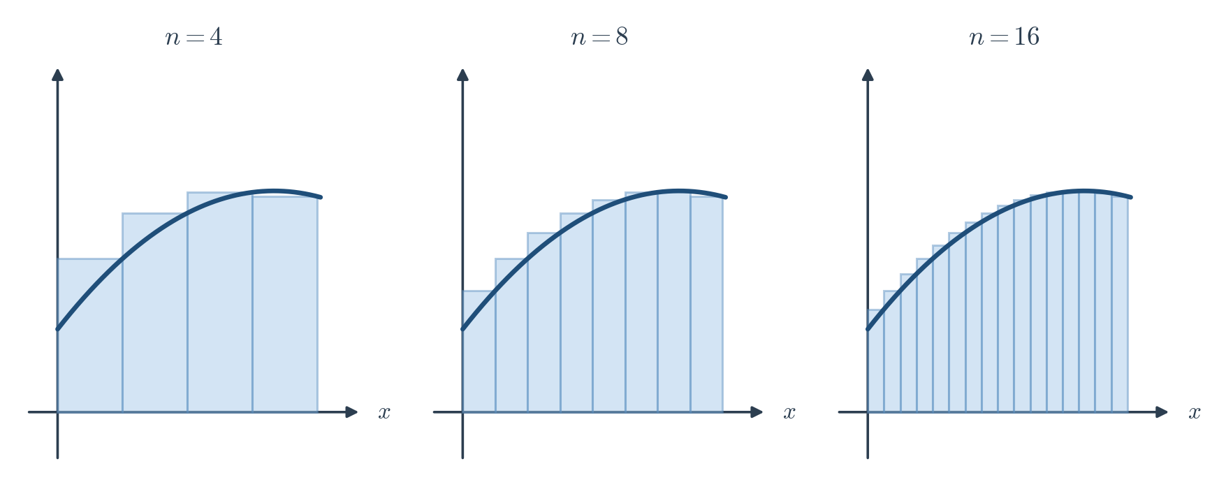
Now take the limit. As $n \to \infty$ the rectangles become infinitely thin, the staircase melts onto the curve, and the approximation becomes the exact area.

The definite integral

The definite integral of $f$ from $a$ to $b$ is the limit of its Riemann sums: $$\int_a^b f(x)\,dx = \lim_{n\to\infty} \sum_{i=1}^{n} f(x_i)\,\Delta x.$$

The notation is a story in itself. The sign $\displaystyle\int$ is an elongated S, for “sum”; it is the $\Sigma$ of the Riemann sum, stretched out as the sum becomes continuous. The $dx$ is the width $\Delta x$ in the limit — the infinitely thin slice. Together, $\int_a^b f(x)\,dx$ reads “sum up $f(x)$ times a sliver of width $dx$, as $x$ runs from $a$ to $b$.” The result is a single number: the area.

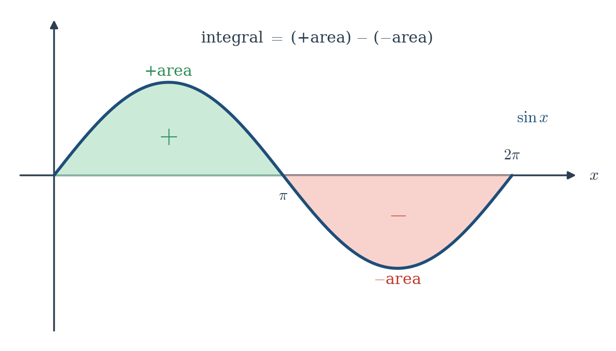
One subtlety: it is signed area. Where $f$ is below the axis, $f(x_i)$ is negative, so those rectangles contribute negatively. The definite integral counts area above the axis as positive and area below as negative. (For distance, this is exactly right — moving backward subtracts.)

Computing one from the definition. Let’s find $\displaystyle\int_0^1 x^2\,dx$ — the area under the parabola from $0$ to $1$ — with nothing but the definition. Slice $[0,1]$ into $n$ pieces of width $\tfrac1n$ and sample at the right edges $x_i = \tfrac{i}{n}$:

$$\sum_{i=1}^{n} \left(\frac{i}{n}\right)^2 \cdot \frac1n = \frac{1}{n^3}\sum_{i=1}^{n} i^2 = \frac{1}{n^3}\cdot\frac{n(n+1)(2n+1)}{6} = \frac{(n+1)(2n+1)}{6n^2}.$$

(We used the sum-of-squares formula $\sum i^2 = \tfrac{n(n+1)(2n+1)}{6}$ from Chapter 1.) As $n\to\infty$, the dominant terms give $\dfrac{2n^2}{6n^2} = \dfrac13$. So $\displaystyle\int_0^1 x^2\,dx = \frac13$. We found the exact area under a parabola by adding up infinitely many rectangles — but it took real work, and we’d have to start over for every new function. Hold that frustration; the next chapter eliminates it entirely.

Properties you’ll use constantly

A few facts follow straight from the definition (sums behave this way, so their limits do too):

• Linearity: $\displaystyle\int_a^b \big[f(x)+g(x)\big]\,dx = \int_a^b f + \int_a^b g$, and $\displaystyle\int_a^b c\,f(x)\,dx = c\int_a^b f$.
• Additivity over intervals: $\displaystyle\int_a^b f + \int_b^c f = \int_a^c f$ — areas of adjacent pieces add.
• A point has no width: $\displaystyle\int_a^a f = 0$.
• Reversing orientation flips the sign: $\displaystyle\int_b^a f = -\int_a^b f$.

All 12 chapters of Calculus I · Foundations · All courses